This package contains various functions to scrape and clean play-by-play data from NHL.com. Season play-by-play data scraped with these functions can be found in the hockeyR-data repository. It also contains functions to scrape data from hockey-reference.com, including standings, player stats, and jersey number history.
Installation
Install the released version of hockeyR from CRAN with:
install.packages("hockeyR")Alternatively, you can install the development version of hockeyR from GitHub with:
# install.packages("devtools")
devtools::install_github("danmorse314/hockeyR")
Usage
Load the package (and any others you might need—for plotting an ice surface I highly recommend the sportyR package).
Loading season play-by-play
The fastest way to load a season’s play-by-play data is through the load_pbp function, which pulls the desired season(s) from hockeyR-data. load_pbp also has the advantage of accepting more explicit values for the seasons desired. For example, if you want to get the play-by-play for the 2020-2021 NHL season, all of load_pbp('2020-2021'), load_pbp('2020-21'), and load_pbp(2021) will get it for you. The option shift_events is a logical value indicating whether or not to load the play-by-play data with specific shift change events. The default is to exclude them, which cuts the size of the data in half and still leaves the most important events like shots, penalties, and faceoffs. Data without shift events does still include columns for players on the ice at the time of each event.
pbp <- load_pbp('2018-19')The available data goes back to the 2010-2011 season as of now, as the NHL JSON source used for this scraper doesn’t include detailed play-by-play prior to that.
All variables available in the raw play-by-play data are included, along with a few extras added on including:
- shot_distance
- shot_angle
- x_fixed
- y_fixed
The shot_distance and shot_angle are measured in feet and degrees, respectively. The variables x_fixed and y_fixed are transformations of the x and y event coordinates such that the home team is always shooting to the right and the away team is always shooting to the left. For full details on the included variables, see the scrape_game documentation.
NEW in hockeyR v1.1.0: Expected Goals
As of hockeyR v1.1.0, a new column has been added to the play-by-play data: Expected goals! The hockeyR package now includes its own public expected goals model, and every unblocked shot in the play-by-play data now has an xg value. A full description of the model, including the code used to construct it and the testing results, can be found in the hockeyR-models repository. Users can now investigate additional statistics, such as player goals above expectation without having to create their own entire model.
pbp %>%
  filter(event_type %in% c("SHOT","MISSED_SHOT","GOAL")) %>%
  filter(season_type == "R" & period_type != "SHOOTOUT") %>%
  group_by(player = event_player_1_name, id = event_player_1_id, season) %>%
  summarize(
    team = last(event_team_abbr),
    goals = sum(event_type == "GOAL"),
    xg = round(sum(xg, na.rm = TRUE),1),
    gax = goals - xg,
    .groups = "drop"
  ) %>%
  arrange(-xg) %>%
  slice(1:10)
#> # A tibble: 10 x 7
#>    player                 id season   team  goals    xg    gax
#>    <chr>               <int> <chr>    <chr> <int> <dbl>  <dbl>
#>  1 John.Tavares      8475166 20182019 TOR      47  40    7
#>  2 Nathan.MacKinnon  8477492 20182019 COL      41  39.1  1.90
#>  3 Tyler.Seguin      8475794 20182019 DAL      33  38.1 -5.1
#>  4 Alex.Ovechkin     8471214 20182019 WSH      51  36.3 14.7
#>  5 Cam.Atkinson      8474715 20182019 CBJ      41  35.2  5.8
#>  6 Connor.McDavid    8478402 20182019 EDM      41  33.9  7.1
#>  7 Brendan.Gallagher 8475848 20182019 MTL      33  33.6 -0.600
#>  8 Patrick.Kane      8474141 20182019 CHI      44  33.5 10.5
#>  9 Sean.Monahan      8477497 20182019 CGY      34  33.2  0.800
#> 10 Sebastian.Aho     8478427 20182019 CAR      30  32.9 -2.9
Shot Plots
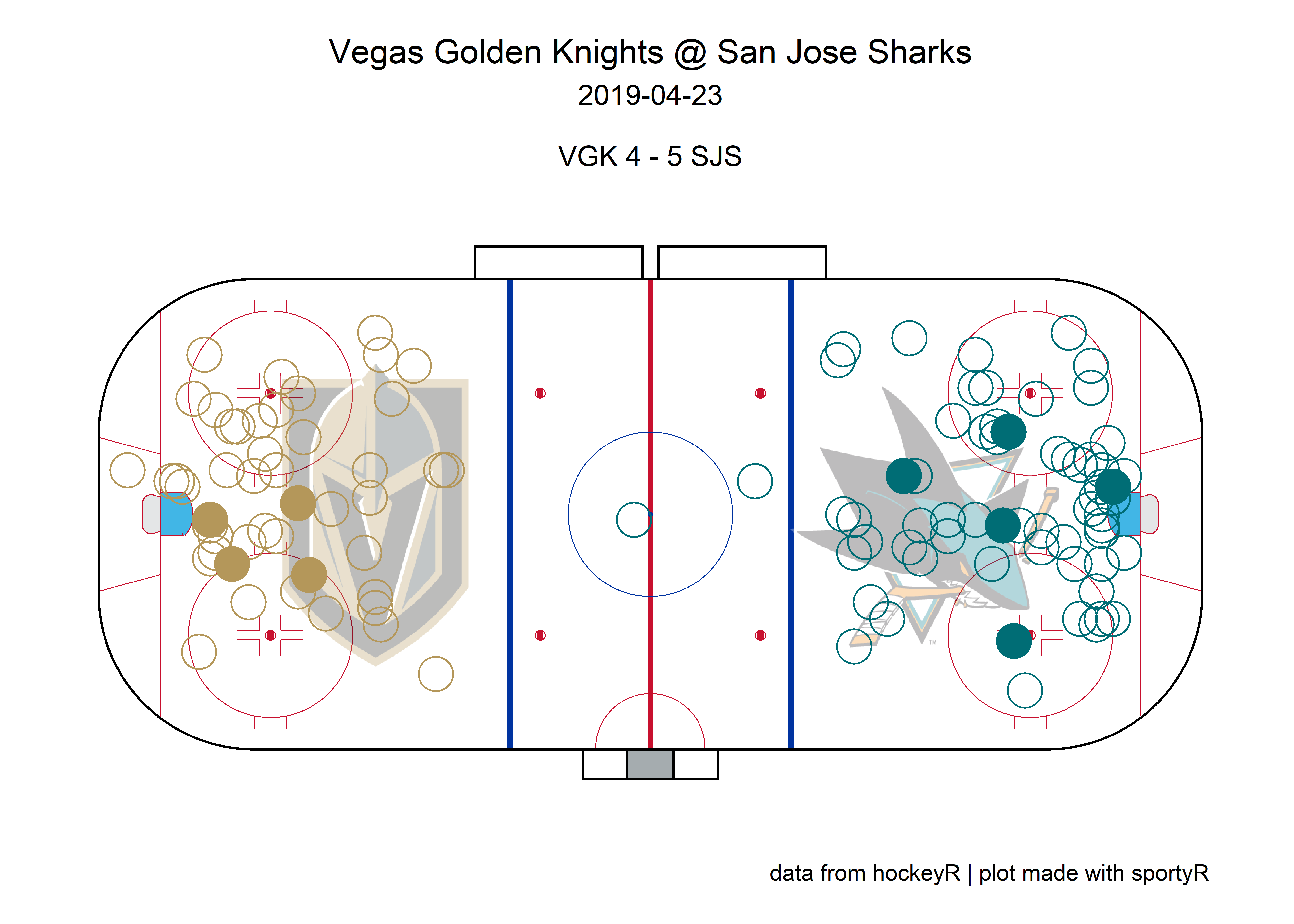
An easy way to create a shot plot is through the sportyR package. You can also use the included team_colors_logos data to add color and team logos to your plots.
# get single game
game <- pbp %>%
  filter(game_date == "2019-04-23" & home_abbreviation == "SJS")

# grab team logos & colors
team_logos <- hockeyR::team_logos_colors %>%
  filter(team_abbr == unique(game$home_abbreviation) | team_abbr == unique(game$away_abbreviation)) %>%
  # add in dummy variables to put logos on the ice
  mutate(x = ifelse(full_team_name == unique(game$home_name), 50, -50),
         y = 0)

# add transparency to logo
transparent <- function(img) {
  magick::image_fx(img, expression = "0.3*a", channel = "alpha")
}

# get only shot events
fenwick_events <- c("MISSED_SHOT","SHOT","GOAL")

shots <- game %>% filter(event_type %in% fenwick_events) %>%
  # adding team colors
  left_join(team_logos, by = c("event_team_abbr" = "team_abbr"))

# create shot plot
geom_hockey("nhl") +
  ggimage::geom_image(
    data = team_logos,
    aes(x = x, y = y, image = team_logo_espn),
    image_fun = transparent, size = 0.22, asp = 2.35
    ) +
  geom_point(
    data = shots,
    aes(x_fixed, y_fixed),
    size = 6,
    color = shots$team_color1,
    shape = ifelse(shots$event_type == "GOAL", 19, 1)
    ) +
  labs(
    title = glue::glue("{unique(game$away_name)} @ {unique(game$home_name)}"),
    subtitle = glue::glue(
    "{unique(game$game_date)}\n
    {unique(shots$away_abbreviation)} {unique(shots$away_final)} - {unique(shots$home_final)} {unique(shots$home_abbreviation)}"
    ),
    caption = "data from hockeyR | plot made with sportyR"
    ) +
  theme(
    plot.title = element_text(hjust = 0.5),
    plot.subtitle = element_text(hjust = 0.5),
    plot.caption = element_text(hjust = .9)
    )
More scraping functions
In addition to the play-by-play data, hockeyR also provides access to a few other endpoints in the NHL’s API. You can scrape the current official rosters for all NHL teams using the get_current_rosters function. This pulls the rosters directly from the NHL at the time you run the function, and will provide the most up-to-date info on team rosters, including player positions, jersey numbers, and player IDs.
rosters <- get_current_rosters()

rosters %>%
  select(player, jersey_number, position, team_abbr, everything()) %>%
  head()
#> # A tibble: 6 x 8
#>   player           jersey_number posit~1 team_~2 playe~3 posit~4 team_id full_~5
#>   <chr>                    <int> <chr>   <chr>     <int> <chr>     <int> <chr>
#> 1 Jonathan Bernier            45 G       NJD     8473541 G             1 New Je~
#> 2 Reilly Walsh                 8 D       NJD     8480054 D             1 New Je~
#> 3 Brendan Smith                2 D       NJD     8474090 D             1 New Je~
#> 4 Tomas Tatar                 90 LW      NJD     8475193 F             1 New Je~
#> 5 Erik Haula                  56 LW      NJD     8475287 F             1 New Je~
#> 6 Ondrej Palat                18 LW      NJD     8476292 F             1 New Je~
#> # ... with abbreviated variable names 1: position, 2: team_abbr, 3: player_id,
#> #   4: position_type, 5: full_team_name
It’s also possible to access the draft selections and order of selections for every NHL Entry Draft back to 1963 (the first year the NHL held an Entry Draft). By default, this function returns only information on the pick number, the team, and the players’ names and player IDs – it runs much faster this way. For more details, including player heights, weights, birthplaces, and amateur teams, set the player_details argument to TRUE.
draft <- get_draft_class(draft_year = 2022, player_details = TRUE)

draft %>%
  select(draft_year, round, pick_overall, full_team_name, player, everything()) %>%
  head()
#> # A tibble: 6 x 24
#>   draft_y~1 round pick_~2 full_~3 player pick_~4 prosp~5 playe~6 first~7 last_~8
#>       <int> <chr>   <int> <chr>   <chr>    <int>   <int> <chr>   <chr>   <chr>
#> 1      2022 1           1 Montré~ Juraj~       1   85964 /api/v~ Juraj   Slafko~
#> 2      2022 1           2 New Je~ Simon~       2   87097 /api/v~ Simon   Nemec
#> 3      2022 1           3 Arizon~ Logan~       3   84987 /api/v~ Logan   Cooley
#> 4      2022 1           4 Seattl~ Shane~       4   85859 /api/v~ Shane   Wright
#> 5      2022 1           5 Philad~ Cutte~       5   90175 /api/v~ Cutter  Gauthi~
#> 6      2022 1           6 Columb~ David~       6   86009 /api/v~ David   Jiricek
#> # ... with 14 more variables: birth_date <chr>, birth_city <chr>,
#> #   birth_country <chr>, height <chr>, weight <int>, shoots_catches <chr>,
#> #   position <chr>, player_id <int>, draft_status <chr>,
#> #   prospect_category <chr>, amateur_team <chr>, amateur_league <chr>,
#> #   position_type <chr>, birth_state_province <chr>, and abbreviated variable
#> #   names 1: draft_year, 2: pick_overall, 3: full_team_name, 4: pick_in_round,
#> #   5: prospect_id, 6: player_link, 7: first_name, 8: last_name
There are also several scrapers designed to pull statistics from hockey-reference.com. For more information on these scrapers and what they can do, please see the Scraping hockey-reference.com vignette.
Future Work
Getting clean data for games going back to the start of the NHL RTSS era (2007-2008 season) is in the works. There are also plans to create a win probability model that would include win probabilities for each play, similar to the win probability model found in the nflfastR package. And of course, scraping the upcoming NHL season and updating the data daily is planned for the 2022-23 season.
Acknowledgments
- Everyone involved in making the nflverse, the premier data source for NFL stats that inspired this whole project
- The Evolving Wild twins, whose old NHL scraper helped enormously in getting player on-ice data joined to the raw play-by-play data in here.
- Tan Ho, whose twitch streams on web scraping and JSON wrangling quite literally took me from 0 web scraping knowledge to building this package